While calculating a peptide’s isoelectric point (pI) and net charge provides a global average of its ionization state, peptide charge distribution reveals the spatial reality of the molecule. In the laboratory, the difference between a soluble, active peptide and an aggregated “ghost peak” often depends on whether charges are distributed evenly or clustered into electrostatic hotspots.
Map Peptide Amphipathicity with Peptalyzer™
Use Peptalyzer™ to generate 3D-oriented Spiral Helical Wheel and β-Strand Zig-Zag projections that help visually identify hidden hydrophobic faces before starting your synthesis.
📘 What will you learn here?
The Physics of Charge Density: Beyond the Net Charge
A peptide is not a uniform “string of beads”; it is a three-dimensional entity where the proximity of ionizable side chains creates local environments that defy global averages.
Net Charge vs. Local Density
A peptide might have a “safe” net charge of +3 at pH 7.0, yet still precipitate in aqueous buffer. This occurs when the basic residues (R, K, or H) are clustered at one terminus, leaving the remainder of the sequence as a long, hydrophobic “grease” patch. Identifying these localized charged patches is essential for predicting surfactant-like behavior and difficult purification.
The Proximity Effect and pKa Shifting
Standard calculators assume each residue behaves in isolation. However, in a real peptide, a Glutamic acid (E) side chain positioned directly next to an Aspartic acid (D) will experience electrostatic repulsion, which can subtly shift their effective pKa values. By visualizing the Charge Topology, chemists can spot these crowded regions where ionization might be inhibited or enhanced by neighboring groups.
Terminal Masking and Electrostatic Orientation
The choice of N-terminal and C-terminal modifications does more than just prevent proteolysis; it fundamentally reorients the peptide’s charge distribution.
- Acetylation (Ac-): Removes the positive charge of the N-terminal amine.
- Amidation (-NH₂): Silences the negative charge of the C-terminal carboxyl. By “silencing” these termini, a chemist can force the peptide to rely solely on its internal side-chain distribution for solubility.
3D Topological Mapping: Seeing the Charge
Peptalyzer™ bridges the gap between a 1D sequence and simplified 3D topology using canonical residue-based models. These visualizations are optimized for sequences between 7 and 40 residues due to model constraints and to maintain scientific accuracy.
The 7–40 Residue Rule: At lengths shorter than 7 residues, secondary structures are rarely stable enough to define a consistent topology. Conversely, beyond 40 residues, the complexity of tertiary folding (the “protein regime”) makes simplified 2D projections of helices or sheets visually cluttered and less predictive for the synthetic chemist.
These topology maps are defined using canonical residue properties derived from Chou–Fasman secondary structure propensities and Eisenberg hydrophobicity values. In Peptalyzer™, noncanonical residues are included only when a chemically defensible canonical analog is defined in the residue library. Because each map depends on specific underlying models, support is feature-dependent: the β-strand map requires Chou–Fasman support, while the helical map requires both Chou–Fasman and Eisenberg compatibility for every residue. Residues without valid mapping block the visualization, while partial-support residues are included only in exploratory mode. As a result, topology visualization with noncanonical sequences is conditional and may be unavailable depending on residue composition. Full details of mapping rules, support levels, and gating behavior are provided in the noncanonical amino acids guide.
Case Study: The Spiral Helical Wheel (The 3D Spiral)
Peptides often exist in a state of conformational competition. As seen in the Magainin 2 example, the Chou-Fasman algorithm may indicate a higher statistical propensity for β-sheets (Max 37.8%) than α-helices (34.7%). Visualizing the sequence through the Spiral Helical Wheel is critical for identifying 3D-oriented face segregation patterns that can influence solubility.
- Chou-Fasman Probability:: The tool displays the Global Compositional Probability (%), warning the chemist if a sequence is prone to structural switching or aggregation.
- Amphipathic Faces: Despite the high β-sheet score, the helical wheel reveals a perfectly organized “charged face” (Lysine residues K4, K10, K11, K14, K15) and a “grease face” (F5, F12, F16, V17).
- Salt-Bridge Detection: The wheel reveals potential salt-bridges (e.g., D→K) that stabilize the helix but may decrease solubility by “masking” the charge from the solvent. However, the wheel highlights spatial proximity between residues at positions i and i+3/4. In Magainin 2, while the K14 and E19 are too far for a direct bridge, the alignment of K11 and K15 on the helical wheel confirms a highly organized charged face. This clustering of like-charges (i→i+4) creates a strong electrostatic dipole that is a hallmark of antimicrobial peptide potency.
Example Sequence (Magainin 2): GIGKFLHSAKKFGKAFVGEIMNS

Case Study: The β-Strand Zig-Zag Map
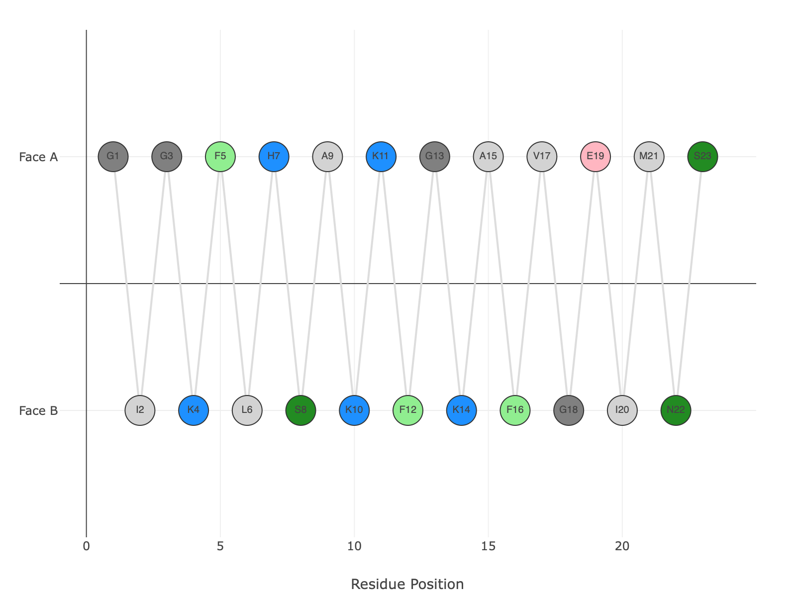
When the Thermodynamic Aggregation Risk stays consistently above the 30% threshold, the β-Strand Zig-Zag Mapbecomes your primary troubleshooting tool for synthesis.
- Peak Aggregation Risk: In this example, the Peak Aggregation Risk (37.8%) triggers a [Monitor Couplings] warning. This tells the chemist that during SPPS, the peptide is likely to aggregate into a β-sheet despite its intended helical function.
- Alternating Topology: By mapping residues to Face A and Face B, the zig-zag view shows exactly where the hydrophobic “stickiness” resides.
- Charge Repulsion as a Tool: For Magainin 2, the map shows that many Lysine charges are on Face B, which helps counteract the hydrophobic clustering on Face A. If all charges were on one face and all hydrophobes on the other, the risk of “ghost peaks” and irreversible aggregation would be significantly higher.
Example Sequence (Magainin 2): GIGKFLHSAKKFGKAFVGEIMNS
Predictive Metrics for Solubility and Interaction
We use the mathematical relationship between charge density and hydrophobicity to provide a diagnostic verdict on peptide behavior.
The Polarity Matrix (H vs. fc)
The Peptalyzer™ Polarity Matrix plots the Charge Fraction (fc) against Total Hydrophobicity (H).
- Intermediate Behavior: A high fc with high H suggests a peptide that may require organic co-solvents like DMSO despite its charged residues.
- The Surfactant Risk: A high fc clustered at one end of the molecule results in a “soapy” peptide that is notoriously difficult to purify via reverse-phase HPLC.
Interaction Potential (Boman Index)
The Boman Index quantifies the potential for protein-protein interactions. A high index indicates that the charge distribution is optimized for binding to other proteins or membranes.
Bench Diagnostics and Troubleshooting
How to use charge distribution to solve real-world synthesis and purification problems.
Selecting Ion-Exchange (IEC) Resins
Don’t just look at the pI; look at the Charged Faces. A peptide with a high local density of Arginine (R) and Lysine (K) on one helical face will bind much more strongly to a Cation Exchange resin than a peptide with the same net charge but a scattered distribution.
Correcting Concentration Errors
Charge density, particularly near aromatic residues (F, W, Y), can interfere with UV concentration checks. For highly charged peptides, rely on the ϵ205 Extinction Coefficient, but be aware that dense charge clusters can cause subtle shifts in backbone absorbance.
Synthesis “Difficult Coupling” Zones
Review the Max β-sheet percentage in the Aggregation Risk section. If your charge distribution map shows no ionizable groups within a 6-residue hydrophobic window, you are significantly more likely to encounter coupling failures during SPPS.
Peptide Charge Distribution — FAQ
Net charge is a global average, but charge distribution dictates physical behavior. Use the Kyte-Doolittle Hydropathy Profile to spot linear grease patches, and the Spiral Helical Wheel or Zig-Zag Mapto identify 3D hydrophobic faces that cause surfactant-like behavior.
Statistical propensity (e.g., Chou-Fasman scores) indicates what a peptide wants to do based on composition. 3D topology (e.g., the Spiral Helical Wheel) visualizes the spatial orientation if that state is adopted. A peptide like Magainin 2 may show a high statistical β-sheet score, yet its functional topology is an amphipathic α-helix.
This range ensures scientific accuracy. Peptides under 7 residues cannot form stable i→i+4 helical turns. Beyond 40 residues, complex tertiary folding makes simplified 2D projections less predictive for synthetic chemistry.
These are segments where aggregation risk exceeds 35%. Lacking ionizable side chains to provide electrostatic repulsion, these regions tend to aggregate into β-sheets on-resin. The Zig-Zag Map helps identify which “Face” drives this stickiness.
References
Lee, J., Shim, J. H., Moon, S., & Kim, G. W. (2022). Helical structure motifs made searchable for functional peptide design. Nature Communications, 13(1), 3769.
- Establishes a searchable framework for identifying helical motifs and spatial amphipathicity to predict the functional and structural behavior of synthetic peptides.
- DOI:10.1038/s41467-022-31553-x
Payliss, B. J., Vogel, J., & Mittermaier, A. K. (2019). Side chain electrostatic interactions and pH-dependent expansion of the intrinsically disordered, highly acidic carboxyl-terminus of γ-tubulin. Protein Science, 28(6), 1095–1105.
- Investigates how localized electrostatic repulsion between neighboring acidic side chains drives conformational expansion and significantly shifts effective pKa values.
- DOI: 10.1002/pro.3618
Meisl, G., Yang, X., Dobson, C. M., Linse, S., & Knowles, T. P. J. (2017). Modulation of electrostatic interactions to reveal a reaction network unifying the aggregation behaviour of the Aβ42 peptide and its variants. Chemical Science, 8(6), 4352–4362.
- Demonstrates that the spatial distribution of charges and ionic strength are the primary regulators of the reaction pathways leading to β-sheet aggregation hotspots.
- DOI: https://doi.org/10.1039/c7sc00215g
Schreier, S., Malavolta, L., & Nakaie, C. R. (2008). Interpretation of the dissolution of insoluble peptide sequences based on the acid-base properties of the solvent. Biopolymers, 90(4), 481–495.
- Explains the biophysical basis of peptide insolubility by analyzing how charge distribution and salt-bridging mask ionizable groups from the solvent.
- DOI:10.1110/ps.051956206